
Why the Area Under a Curve Equals 1
Why every probability density curve encloses an area of exactly 1, and how area under the curve becomes probability for a continuous random variable.
Selected from the official eduvids YouTube channel and presented here as an example of the product's output.
Transcript
Roll a standard six-sided die and before it lands, ask which number is guaranteed to appear. None of them is guaranteed, but the chance of each face landing face up is not random. Every possible result has a number attached to it, measuring how often it should occur. When you list every possible outcome alongside its exact likelihood, you get a probability distribution.
Think of probability as one whole pound of clay spread across every possible reality. For our rolling die, there are six separate landing spots where that clay can settle. Each numbered face from 1 to six receives exactly one sixth of the total pile. This recipe for assigning probability to isolated values is called a probability mass function or PMF.
Because something has to happen, adding the heights of all six bars gives exactly one. To find the probability of rolling an even number, just gather the bars for 2, 4, and six. 1 16th added three times gives 36 or exactly 1/2. What happens if we shrink the game down to just two possible outcomes?
Imagine flipping a single biased coin that lands on heads with probability P. The only other outcome is tails, which must take whatever is left of our total probability. That leaves tails with an exact probability of 1 minus P. This single yes or no test is called a Berni distribution.
If you count heads as one and tails as zero, your average outcome over time is simply P. Now repeat that coin toss five times in a row and ask for exactly three heads. Each specific sequence with three heads, like heads, heads, heads, tails, tails, has the same exact chance. That chance is P cubed multiplied by 1 minus P ^ 2.
Many different orderings produce three heads. So we must count how many paths lead there. The combinations formula counts how many ways three heads can be chosen from five slots. 10 distinct arrangements exist, each carrying the identical slice of probability.
Multiplying the number of paths by the chance of each path gives the binomial distribution. Sometimes instead of counting flips, you count events that arrive throughout a stretch of time. Imagine waiting for incoming emails where you average two messages every single hour. This hourly arrival rate gets labeled with the Greek letter lambda.
Events arrive independently and unpredictably. Yet their total tally follows a reliable pattern. The pson formula gives the exact chance of seeing any count like four emails in that hour. It multiplies lambda to the 4th power by e to the negative lambda / 4 factorial.
Plugging in two for lambda shows there is roughly a 9% chance of getting four messages. Here is the catch. What happens when outcomes are not separate steps but a continuous spectrum? If you measure human height or bus arrival times, the number of possible outcomes becomes infinite.
Because infinitely many points exist, the probability of hitting any single exact number drops to zero. We cannot use bars anymore. So we draw a smooth curve called a probability density function. This density curve abbreviated as PDF never gives probabilities through its vertical height.
Instead, probability limps entirely in the area underneath the curve between two chosen values. The total area under the entire curve stretched across all real numbers always equals 1. To track how this area accumulates from left to right, we use a cumulative distribution function. This accumulating curve or CDF tells you the chance of falling below any target value.
The simplest continuous shape is a uniform distribution spreading probability evenly across an interval that a bus arriving anywhere between 0 and 5 minutes with totally flat likelihood. The curve forms a flat rectangle from 0 to 5 with a constant height of 1/5. The area of that whole rectangle equals width 5 * height 1/5 which is 1. The chance the bus arrives between 2 and 3 minutes is width 1 * height 1/5.
Nature, however, rarely spreads things out in perfect flat rectangles. Measurements like height, test scores, and sensor noise gather around a central average and taper off symmetrically. This bell-shaped curve is the normal distribution centered on its mean value, mu. The width of the bell depends on sigma, the standard deviation, which measures how widely points spread.
About 68% of all outcomes land within one standard deviation of the center. Pushing out two standard deviations captures roughly 90 miss% of all possible values. Other continuous processes do not balance around a peak but decay immediately from the start. The exponential distribution models the waiting time until the next random event occurs.
If buses arrive with an average weight of 5 minutes, the arrival rate lambda is 0. 2. The height of the curve drops steadily as time passes governed by e to the negative lambda x. Using its cumulative formula, the chance of waiting less than 3 minutes is about 45%.
A common trap is assuming the height of a continuous curve cannot ever exceed the number one. Because height is density rather than probability, a very narrow curve can shoot up past one easily. As long as the total area under that narrow spike stays equal to one, the rules hold true. For distinct counts, you add discrete bars, but for smooth continuous flows, you integrate under the curve.
Test these patterns against real data and the world stops looking unpredictable. Continue with our previous video, why overlapping events break naive edition. The link is in the description and top comment.
More visual explanations
 Video
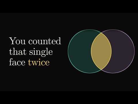
VideoWhy Overlapping Events Break Naive Addition
Why P(A or B) is not simply P(A) + P(B) when events overlap, and how the inclusion–exclusion principle removes the outcomes counted twice.
 Short
ShortWhat Is an Integral? Calculus Explained Visually
See how Riemann sums turn infinitely thin slices into area, then connect that idea to antiderivatives through the fundamental theorem of calculus.
 Video
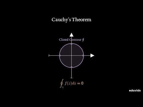
VideoComplex Integration Visualized From First Principles
Extend integration into the complex plane using paths, parameterization, Cauchy’s theorem and the residue theorem.